
A tribute to Douglas Adams
Sources:
Neil Turok's Lecture on Dark Matter and The Astonishing Simplicity of Everything Garrett Lisi's Ted Talk and Lecture on the E8 Lie Group, and Particle Physics
The Beginning.
The Universe is ≈ fourteen billion years old. Since the moment of the big bang, energy and time have been the factors shaping the Universe. Astoundingly, life has pulled a fast one on us. The Universe, at it's largest and smalles scales is actually quite simple. It is the middle part known as life, where we reside, that is most complicated. Our birth and death are understood, and our lives are chaotic.The Hitchhiker's Guide to the Galaxy:
"The story so far: In the beginning, the Universe was created. This has made a lot of people very angry and has been widely regarded as a bad move."
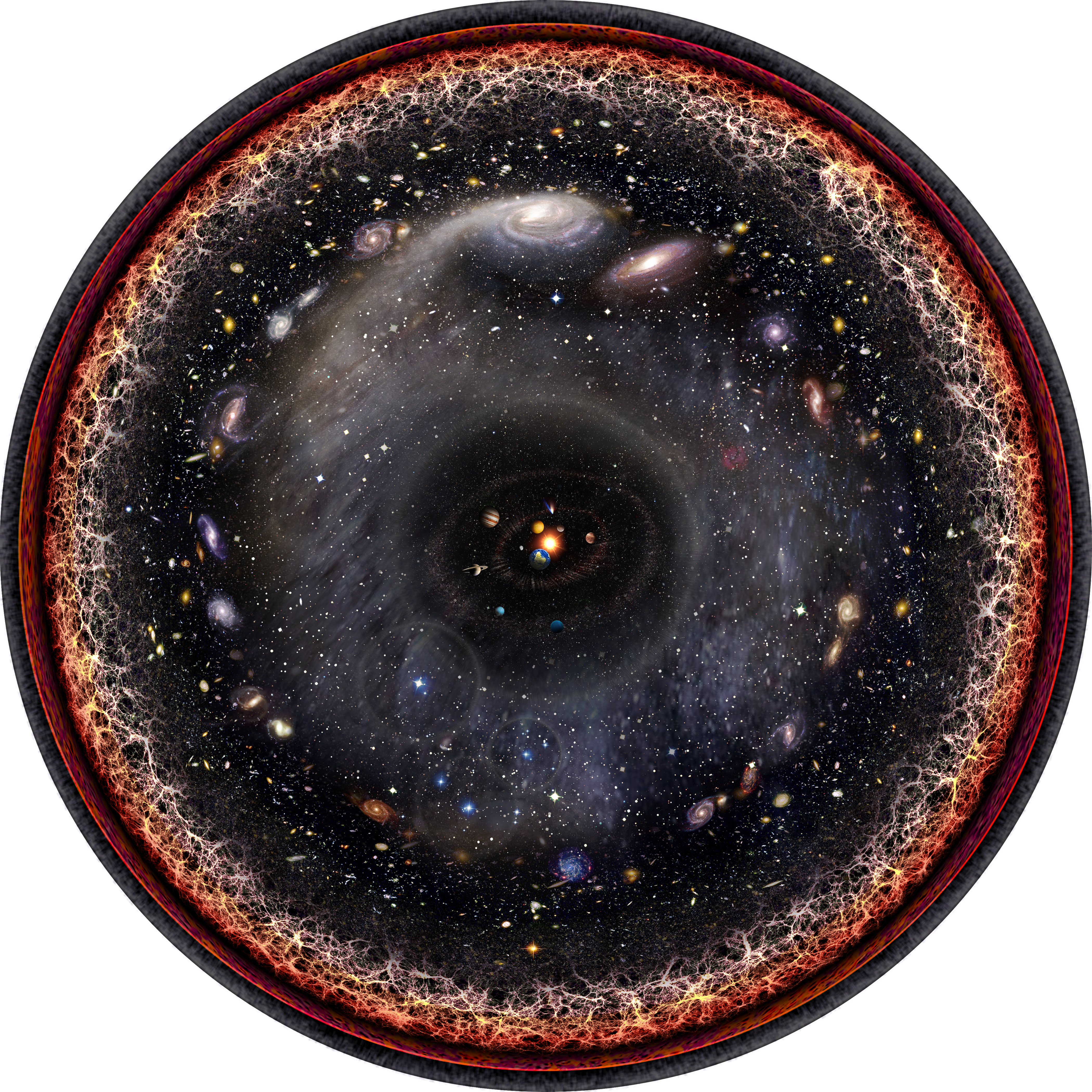
An illustration of the observable Universe on a logarithmic scale as depicted by Pablo Carlos Budassi.
Observable Universe
As you look up into the night sky, information about small and large stars, near and far, enter your eyes. This information is interpreted by your visual cortex, and you see the stars. One unintuitive notion about star gazing, is that as you look outwards into space, you are actually looking backwards in time. This is because light takes time to reach us.
As we travel backwards and away from the earth in time in the illustration above: the sun is in the middle orbited by the earth in our solar system, there is a vast expanst of space full of galaxies, and the cosmic web.
The cosmic web is the structure of the Universe as it began to form at early times. After the cosmic web is a bright red ring, which signifies the hot plasma of the early Universe. Beyond this portion of the Universe is the Dark Ages; the information currently unavailable to us due to limitations in technology. When we develop ways to probe beyond the red ring of our Universe such as gravitational waves, we will be able to see how our Universe actually began.
Scale
The picture above depicts objects with a logarithmic scale. This means that the objects are scaled relative to their distances away from eachother and relative to their size so there is uniformity when you are comparing distances and sizes. If you examine the picture above, you will notice that there is quite a bit of empty space. This space is referred to as Dark Energy. Dark Energy is responsible for the acceleration and the expansion of the Universe. As the Universe expands, information moves away from us, and reaches a point past which it is unobservable. There is a scale associated with the observable Universe based on this Dark Energy, and it is around the order of 1025 in our picture.
The smallest scale we can observe is the point right at the end of our picture. This scale is referred to as the Planck Scale. If we were to go backwards in time and try to fit a light wave into a singularity of this size, it would create a blackhole because there is so much energy being shoved into a small space. This order is around 10-35.
The size of an individual cell relative to this scale is about 10-5. This puts human beings about exactly in the geometric mean, or in the middle of the scale of reality.
Not only do we reside in the perfect scale to observe the Universe, it turns out that things at the largest scale, and things at the smallest scale are actually the easiest things about the Universe to understand as well.
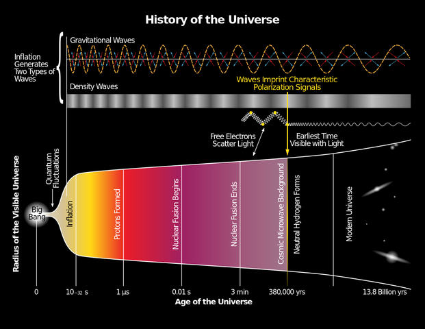
Shape
If you look at any region of space, you will find that it contains a history with the shape depicted above. All of space came from a singularity, resulting in the Big Bang. As you trace the space backwards in time it shrinks into nothing, and as you move forward in time, space is expanded by the Dark Energy.
Synchronicity
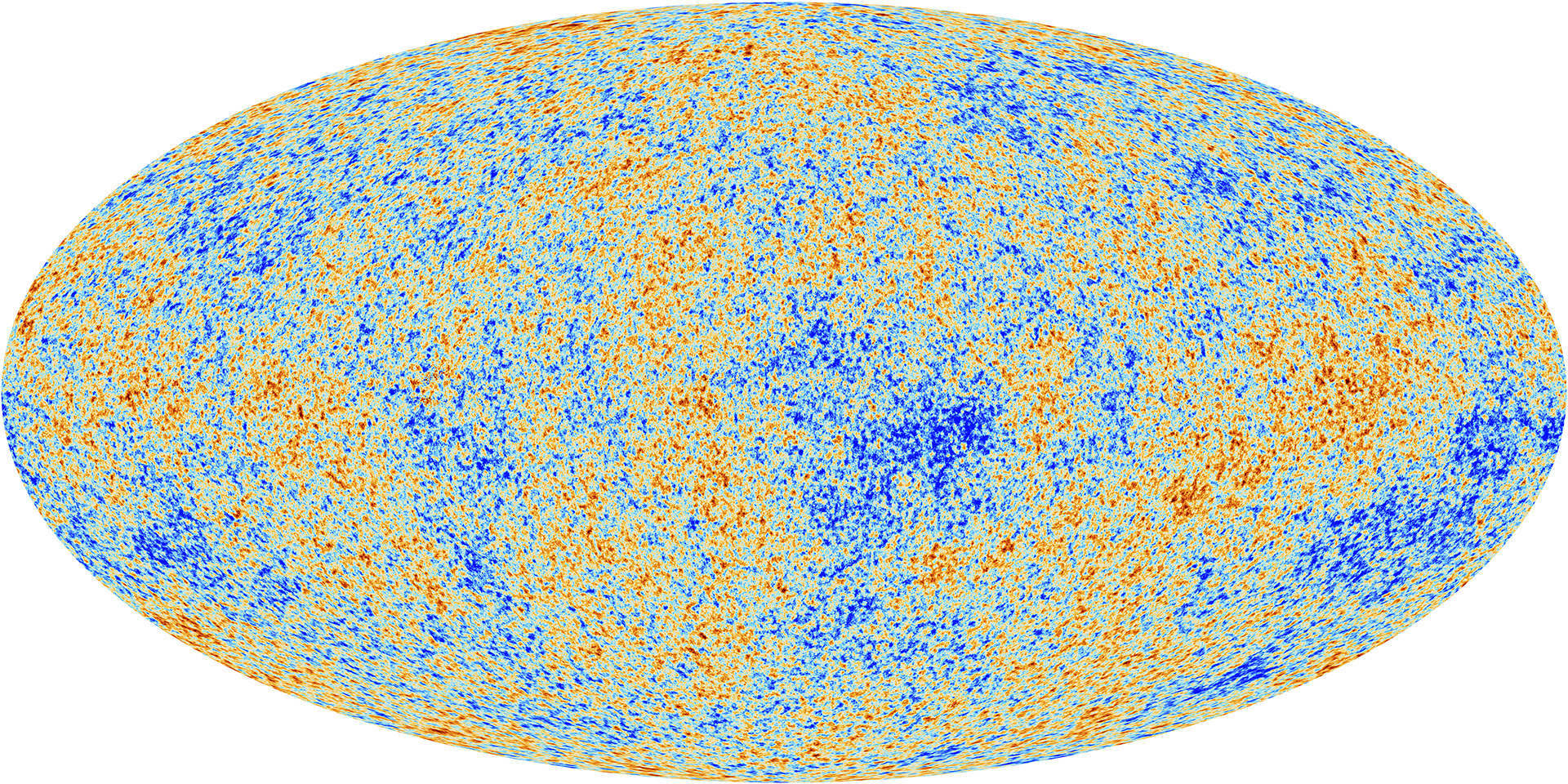
The picture above is courtesy of the Planck Satellite. It depicts the spherical sky above us in terms of variation in density. These variations in density create a variation in temperature because things emit radiation. These variations in temperature are only one part in one hundred thousand from place to place, making them very uniform. The second interesting thing about this picture is that it depicts synchronicity.
If you strike a bell, all of the sound waves are synchronized because they all got excited at the same time. If you look at the graph produced by the sound waves, you can see this pattern and you can detect that it was struck at one moment.
This is what happened in our Universe. All of the information is uniform in the picture from the Planck Satellite because all of the light waves were excited at the same moment, the big bang, oscilated a certain number of times, and reached the satellite. You cannot interpret this simply from the picture, but if you perform a fourier analysis (and add together the waves of different wavelengths) on the variations of temperature, you find the amplitude peaks reach their maximum, and decrease just like sound waves in a bell.
It turns out the only number we need to describe the rest of the Universe is the scalar for Dark Energy, one part in one hundred thousand.
Scalars

A scalar is a number without direction. Another word for this is a magnitude. Real numbers were the first scalars that were used by humans. We know these as 1, 2, 3, 4, 5, 6, 7, 8, 9, 10 and so forth. Let's use scalars to explore the functionality of python considering they have been around since we could rub two sticks together.
#This is a comment, comments are just text that you use to describe your program.
#In python, the # symbol specifies a comment.

#Our first step is to import pylab inline.
%pylab inline
#Next, we simply assign our scalar a value like we would on paper in pseudo code.
s = 1

#This stores a variable in the computer's memory that we can now access.
#As an example, if we want to print the value of S, we simply write...
print(s)
#Additionally, we can take advantage of pylab's inline functionality to print s.
s
#You can add two scalars together
s+s
#Or subtract scalars
s-s
#Multipy scalars
s*2
#And divide scalars
2 // s
Notice that I used two division symbols above. When you use double division symbols, //, it specifies integer division.
#And one division sign divides while including decimals
e/e
#Absolute value
abs(s)
#s to the power of s
pow(s, s)
s**s
The next, most important and often unintuitive operator is modulus. Modulus in python is executed with the % operand, and you will recognize its importance almost immediately if you have ever been rock climbing, got your hand trapped in a crevace, and had to convert hours to days...
day = 24
hours = 127
print(hours/day)
print(hours % day)
print(hours,"hours is:",hours//day,"Days and",hours%day,"hours.")
As you can see, 24 does not divide evenly into 127. When we do division, we find the answer to be 5.29 days. This does not really help us if we want to format the output as days and hours. One way to fix this is to use modulus. Modulus returns the remainder of a division operation. In this case, 127 hours is made of 5 days, with a remainder of 7 hours.
#Numeric Data Types

#Integer (as of python 3, ints are basically longs so there is no longer a long primitive datatype...)
s = 1
print(type(s))

#Float
s = float(s)
print(type(s))

#Complex (or lateral if you want to be esoteric)
s = complex(s)
print(type(s))


#String (more correctly a list of characters, or a sequence in python 3 syntax)
s = str(s)
print(type(s))
s
Let's examine the output of the cell above. Why would the answer be '(1 + 0j)'? Well, first we converted x to a float, making it 1.0, next we converted it to a complex number, which is horribly named because it just means our number has a component that lies on a different axis in our number space... hence + 0j. Next we converted the number to a list of hexadecimal 1's and 0's that the compliler interpreted as the characters (1 + 0j).
#Strings
hello = "Hello"
world = " World"

print(hello + world)
Circuits
"An electric circuit is in many ways similar to your circulatory system. Your blood vessels, arteries, veins and capillaries are like the wires in a circuit. The blood vessels carry the flow of blood through your body. The wires in a circuit carry the electric current to various parts of an electrical or electronic system.-How Circuits Work
Just as your heart produces the pressure to make blood circulate, a battery or generator produces the pressure or force to push electrons around a circuit. Voltage is the force and is measured in volts (V). A typical flashlight battery produces 1.5V, and the standard household electrical voltage is 110V or 220V."
The basis of all logic in a computer is the transistor. Every computer chip has an insane number of transistors. Transistors are typically made of silicon, which as you may know does not normally allow electricity to flow through it. Silicon is therefore considered a semiconductor. By doping silicon with different materials, you can get it to behave more like a conductor, or more like a resistor. Typically, an N-type semiconductor carries an electric current out, and a P-type semiconductor carries current in. The circuit below depicts a diode with the N-type semiconductor as the triangle, and the P-type semiconductor as the line.
 If you toyed around with an Arduino, you may have used the DC motor in one of your circuits. One lesson that you quickly learn is that as the circuit is broken, the motor still retains a bit of angular momentum. This causes the motor to continue to spin, and induct a current back through the circuit, causing a short. This is why induction motors typically have diodes before them. Diodes direct the current in one direction using semiconductors. To create a diode, you simply stack an N-type on top of a P-type semiconductor!
A transistor is a bit more complicated, but relax, programming is never more challenging than a 1 or a 0 unless you are using a quantum computer. A transistor is made up of a base current, that is either on or off, and a stack of PNP type semiconductors. When a current is applied to the base, there is an amplified current, and when there is no current to the base, there is a low current output. An amplified current output corresponds to a 1, and a low current output corresponds to a 0.
![]()
![]()
The above animation from circuitsgallery.com, is a great way to visualize what is happening in a transistor. When the switch is not activated there is a small current in the circuit that increases the amplitude of the transistor firing a 1 to start the motor, but is not strong enough to trip the transistor. When the switch is activated, the base current is applied to the transistor and completes the circuit! On an Arduino this is similar to sending 1's and 0's through serial communication to start a motor.
This is the concept behind logic. A 1, or a 0. The hard disk of your computer is made up of millions of molecules that are positively or negatively charged, indicating a 1 or a 0 in memory. Additionally, every instruction on your cpu is at it's core a combination of 1's and 0's. As the read/write head of your computer searches the hard disk, it reads or writes a 1 or a 0 with an electric charge. The game of computer science is to figure out the best ways to manipulate electrons, 1's and 0's to complete tasks and model the real world to solve problems.
Logic Gates
By combining transistors, we can model many different types of complex circuits and logic gates.
Python has three built in logic gates, or boolean operations.
| x or y | if x is false, then y, else x |
| x and y | if x is false, then x, else y |
| not x | if x is false, then True, else False |
Let's define our first function in python to test the positivities of two electrons using the python built in boolean operators.
def testOr(e1, e2):
    return e1 or e2
e1 = 1
e2 = 1

print(testOr(e1, e2))

e1 = 1
e2 = 0
print(testOr(e1, e2))

e1 = 0
e2 = 1
print(testOr(e1, e2))

e1 = 0
e2 = 0
print(testOr(e1, e2))
def testAnd(e1, e2):
    return e1 and e2
e1 = 1
e2 = 1

print(testOr(e1, e2))

e1 = 1
e2 = 0
print(testOr(e1, e2))

e1 = 0
e2 = 1
print(testOr(e1, e2))

e1 = 0
e2 = 0
print(testOr(e1, e2))
def testNot(e1):
    return not e1

e1 = 1
print(testNot(e1))

e2 = 0
print(testNot(e1))
As you can see, the or operators are working perfectly. Examine the above logic in the table yourself to verify this.
Arrays
Say we have some data corresponding to 1's and 0's. How would we create a mental model of that and translate it to python? Well, one way to do this is to create what is called a list. A list is just what it sounds like, a list of stuff. Your stuff can be anything from a string (words), an integer, a double (has decimal points), to an object (an abstract representation of data). Most other languages refer to this data structure as an array, because in mathematics a one dimensional list of stuff is considered an array.
#Array
Data = [1,0,1,1,0]

#Function
def checkData(d):

    #For Loop
    for n in range(len(d)):

        #Conditional Statement
        if d[n] == 1:

            #Input/Output
            print("Value", n,"is 1")

#Pass data to function
checkData(Data)

#Input/Output
print(Data)
#Another way to specify an array within Ipthon is with numpy
import numpy as np

Data = np.array([1,0,1,1,0])
checkData(Data)
print(Data)
Here are some basic list operations...
#Initialize a list
mylist = []

#Add something to the end
mylist.append(1)
mylist.append(2)
mylist.append(3)

#Print and access specific elements in the list
print(mylist[0])
print(mylist[1])
print(mylist[2])

#Iterate through list
for x in mylist:
    print (x)


#Get size of list
print("Length: ",len(mylist))
Loops
primes = [2, 3, 5, 7]
Python offers many different types of loops, or ways to iterate over data. This is similar to the Σ operator in mathematics.
#For Loop
for prime in primes:
    print (prime)
#For Loop using length of list (or array)... in numpy syntax is array.len I believe.
for x in range(len(primes)):
    print (primes[x])
#While Loop
count = 0
while count < len(primes):
    print (primes[count])
    count += 1  # This is the same as count = count + 1
#Break Statements

# Prints out first three primes
count = 0
while True:
    print(primes[count])
    count += 1
    if count >= 3:
        break

print("\n\n")

# Prints out only odd primes
for x in range(len(primes)):
    # Check if x is even
    if primes[x] % 2 == 0:
        continue
    print(primes[x])
#Else

# Prints out four primes
count=0
while(count<4):
    print(primes[count])
    count +=1
else:
    print("count value reached %d" %(count))


print("\n\n")


for i in range(1,len(primes)):
    if(i%7==0):
        break
    print(primes[i])
else:
    print("Array element",primes[i]+1,"is not printed\
 because for loop is terminated because of break but not due to fail in condition")
Graphs
Graphs are incredibly important tools in computer programming because they allow you to visualize what is going on. Let's graph a simple line.
#Import numpy(a matrix library) and matplotlib (a graphing library)
import numpy as np
import matplotlib.pyplot as plt

#Set up our data.

#An easy way to represent a line in matplotlib is by using numpy.linspace().
#linspace creates a sample space of points, and then is supplied start and stop values for
#the line length. Our line would represent the number 1 in 1 dimension.
x = np.linspace(0, 1)
y = np.linspace(0,1)

line, = plt.plot(x, y, linewidth=2)

plt.show()

Spiral of Theodorus
Although Theodorus' work was lost, Plato catalogued it extensively. Theodorus came up with what I consider to be one of the most important concepts in math, the spiral of Theodorus. Picture yourself as an ancient greek, whose only tools are a sandbox and two sticks of equal length. Theodorus found that if you place the two sticks at right angles, you can derive all kinds of mathematical concepts.

If we label our sides a, b, and c we can remodel the function for the spiral of Theodorus.
#Spiral of Theodorus

#Define a function that will print the results of the Spiral of Theodorus
#n = the number of triangles you want to step through
def spiralOfTheodorus(n):

    #A simple for loop that loops through n, incrementing i upon execution of the loop
    for i in range(n):

        #Side a = 1
        a = 1

        #Side b = sqrt(n)
        b = numpy.sqrt(i)

        #Side c = sqrt(n+1)
        c = numpy.sqrt(i + 1)

        #Print the output
        print("Triangle:",i+1," a:",a," b:",b," c:",c)

#Execute the function
spiralOfTheodorus(17)
There is a historical signifigance for why I chose 17 as the number of triangles, but I will leave that up to the reader to figure out. We can test how our function performed by checking the last triangle.
print("a =",1,"b =",np.sqrt(16),"c =",np.sqrt(17))
Pythagorean Theorem
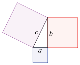
Pythagorus built upon the Spiral of Theodorus, and created the Pythagorean Theorem. Pythagorus found that if he took three squares of sides equal length, he could describe all kinds of mathematics. Most importantly he proved that a2 + b2 = c2.
A square is defined as having sides of equal length. To find the area of a square, we simply "square" the length of one of the sides. If a = 1, a2 = 1. Additionally, if we add the areas of squares a and b, we get the area of square c. This is the basis of the pythagorean theorem, and we can model it quite simply in python.
#Pythagorean Theorem

#Define a function that will print the results of the pythagorean theorem
#This function takes an argument for the length of a and b, and calculates c
def pythagoreanTheorem(a,b):

    #If a^2 + b^2 = c^2, using simple algebra c = sqrt(a^2+b^2)
    c = np.sqrt((a**2)+(b**2))

    #Print a, b, c
    print("a =",a,"b =",b,"c =",c)

#Execute function
pythagoreanTheorem(1,2)
We can test our results as follows.
1. If a2 + b2 = c2, then using simple algebra,
2. c = √ a2 + b2
3. a = 1, b = 2
4. c = √ 12 + 22
4. c = √ 5
print(np.sqrt(5))
Imaginary Numbers
i2 = -1
Ancient civilizations really only cared about natural numbers like 1, 2, and 3. This is because the only things humans needed to do back then was add and subtract stuff. Then the Egyptians expanded on this idea to facilitate monetary transactions by inventing fractions. The next big innovation in the number line was 0 and negative numbers with the invention of debt.
Around five centuries ago, a mathematician by the name of Del Ferro was playing around with the quadratic formula trying to find an equation to cubic functions. At that time, mathematicians would hold duels, and they made money by winning these math duels. Del Ferro successfully found an equation for cubic functions, and kept this equation secret in order to win. The only problem was that his equation did not work for certain numbers due to square roots of negatives.
Del Ferro kept his formula secret to his dying day, on which he told he passed his knowledge to his only student Foir. Foir, with his new formula got cocky and challenged Fontana Tartaglia, another respected mathematician to a duel believing he would win. Tartaglia already claimed he could solve cubic functions, but he was lying. Before the match however, he actually figured it out and beat Foir.
Tartaglia ended up sharing his and Foir's secret formula for cubics under pressure from Cardan, who discovered Del Ferro's original work and decided it was not a big deal for him to publish Del Ferro's work to the public. It was not until another generation of mathematicians that Bombelli, Cardan's student made significant strides with the cubic function.
Bombelli is credited with being one of the first mathematicians to allow square roots of negatives to exist in his equation, or the imaginary number. Additionally this allowed him to find the solution to Cardan's problem. Bombelli never gave his work any credit however, and regarded it as sophistry.
A century later, Euler started using i in his algebra, and made what is regarded as the most important discovery in mathematics, solving the imaginary number problem.
If we imagine a number, x as a scalar, and add an imaginary component iy, we can enlarge our space of numbers. Now numbers can have a real part, and an imaginary part and are two dimensional. In other words, we can do a scalar transformation of x along the number line, and we can also do a scalar transformation in the direction of iy.
Using pythagorus' theorem, and it's derived geometry, we can now make a model of a complex number. Our graphing library has a nice circular graph that takes polar coordinates, so we are going to have to convert our point to polar coordinates before we can graph it.
#Plot a 2d number

#Convert from cartesian to polar coordinates
#r = sqrt(x^2 + iy^2)
#theta = tan^-1(iy/x)

#x
x = 1

#imaginary number
i = 1

#y
y = 1

#radius conversion from x and y
r = np.sqrt((x**2)+(y**2))

#check radius
print("sqrt(2) =",np.sqrt(2))
print(r)

#theta conversion from x and y
theta = np.arctan2(y, x)

#check theta
print(theta)

#graph area
area = 100*r**2

#polar coordinates
ax = plt.subplot(111, projection='polar')

#plot number: theta = angle, r = radius, c = color, s = size
c = plt.scatter(theta, r, c='red', s=area)

#set the alpha channel (transparency)
c.set_alpha(0.75)

#show the plot
plt.show()

To make sure our graph is correct, we can use some simple logic. If we look at the Spiral of Theodorus, we will notice that angles of 45 degrees are special because sides a and b are equal. For our graph, we made sides a and b equal to 1. The Spiral of Theodorus, and geometry from the Pythagorean theorem says that side c, or in our case our radius, should be equal to √ 12 + 12 , or more simply, √ 2
print("Our radius is,",r,"The square root of 2 is,",np.sqrt(2))
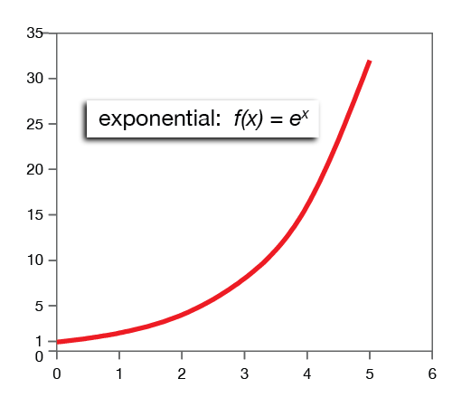
The Exponential Function
The most brilliant mathematician of the eighteenth century was Leonhard Euler. Euler is credited for some of the most amazing proofs in mathematics, and specifically, the invention of the Euler number, e. e is the number that describes exponential growth. Exponential growth is quite intuitive. For example, if you have bacteria that multiply exponentially over time, their graph would look like the one below.
Let's see if we can model exponential growth using Python.
#Exponential Growth

#Import dependencies for animations
from JSAnimation.IPython_display import display_animation
import matplotlib.animation as animation


#Define a callback function for our model data
def modelData():

    #define parameters

    #length of time
    t_max = 10.0

    #change in time
    dt = 0.1

    #x initial state
    x = 0.0

    #time initial state
    t = 0.0

    #update parameters
    while t < t_max:

        #x = e^t
        x = np.exp(t)

        #increment time
        t = t + dt

        #return parameters
        yield x, t

#Define our model
def modelPoints(modelData):

    #set x and t
    x, t = modelData[0], modelData[1]

    #set text displaying time
    time_text.set_text(time_template%(t))

    #pass data to line object
    line.set_data(t, x)

    #return line for matplotlib animation and time text
    return line, time_text

#Create a new plot
#fig = plt.figure()

#Add axes
#ax = fig.add_subplot(111)

#Plot line (empty x, empty y, red circles, 10 miliseconds)
#line, = ax.plot([], [], 'ro', ms=10)

#Set y axes
#ax.set_ylim(1, 22026)

#Set x axes
#ax.set_xlim(0, 10)

#Set time display format
#time_template = 'Time = %.1f s'

#Initialize time text
#time_text = ax.text(0.05, 0.9, '', transform=ax.transAxes)

#Animate
#anim = animation.FuncAnimation(fig, modelPoints, modelData, blit=True, interval=10, repeat=True)

#Display in javascript
#display_animation(anim, default_mode='reflect')
#print(mpl.__version__)
#anim.save('exponentialFunction.gif', writer='imagemagick')
We can easily validate our animation by simply plugging t into the exponential function. In our case, f(x) = et, and finding the value at t = 10.
print("e^10 =",np.exp(10))
If you examine the last frame of our animation, you will see the point is at (t=10, x=22026), accounting for a small error in the image scale between time and x.
Waves
Euler, being the inventor of the euler number, thought it would be a great idea to see what happened if he applied his number to imaginary numbers. It turns out, that if you exponentiate the imaginary number, really cool things happen.

Euler found that if you grow exponentially to the imaginary number multiplied by an angle, you can describe rotations around a circle. For instance:
1. If eiπ = cos(π) + isin(π), pi being in radians,
2. cos(π) = -1,
3. sin(π) = 0,
4. eiπ = -1....or in other words, a 180 degree rotation.
As theta iterates, a point with a corresponding complex number would rotate around the circle. It's real part would go back and forth, or oscillate, much like many things around us in nature.
Let's model this behavior by creating a program that displays two graphs of three points.
Graph 1:
Point 1, labeled in red, will correspond to the real and imaginary parts of our complex number. Point 2, labeled in blue, will correspond to the real part.
Graph 2:
Point 3, labeled in green, will correspond to a sinusoidal wave with the real part of our function as it's amplitude.
#Define a callback function for our model data
def modelData():

    #define parameters

    #length of time
    t_max = 10.0

    #change in time
    dt = 0.1

    #time initial state
    t = 0.0

    #update parameters
    while t < t_max:

        #theta
        theta = (t * 4) / (2*np.pi)

        #radius
        r = 1

        #increment time
        t = t + dt

        #return parameters
        yield r, theta, t

#Define our model
def modelPoints(modelData):

    #set r, theta, and t
    r, theta, t = modelData[0], modelData[1],modelData[2]

    #pass data to line objects

    #A revolution around the circle corresponding to the complex plane
    line1.set_data(theta,r)

    #An oscillation between -1 and 1 depicting the real part
    line2.set_data(0,np.cos(theta))

    #A wave using the real part for amplitude
    line3.set_data(np.cos(theta)/2,t)

    #return line for matplotlib animation and time text
    return line1, line2, line3

#Create a new plot
#fig = plt.figure(1)

#Add wave subplot
#ax = fig.add_subplot(211)

#Set y axes
#ax.set_ylim(0,10)

#Set x axes
#ax.set_xlim(-1, 1)

#Plot wave
#line3, = ax.plot([],[], 'go', ms=10)

#Add polar subplot
#ax = fig.add_subplot(212, projection='polar')

#Plot line (empty x, empty y, red circles, 10 miliseconds)
#line1, = ax.plot([], [], 'ro', ms=10)

#Plot line (empty x, empty y, blue circles, 10 miliseconds)
#line2, = ax.plot([], [], 'bo', ms=10)

#Set y axes
#ax.set_ylim(0,1)

#Set x axes
#ax.set_xlim(0, 2*np.pi)

#Animate
#anim = animation.FuncAnimation(fig, modelPoints, modelData, blit=False, interval=10, repeat=True)

#Display in javascript
#display_animation(anim, default_mode='loop')

#anim.save('wave.gif', writer='imagemagick')
Light
When Maxwell discovered his equations of electricity and magnetism, the consequence was that he could describe light using waves.
In the animation above, the blue arrows are the magnetic field, the red arrows are the electric field, and this field pattern moves along space-time at the speed of light.
What is interesting about Maxwell's equations is that they have no scale. You can take a light wave and shrink it down to an x-ray or gamma ray, or you can scale it up to radio waves and they all obey the same equations.
We can model a light wave by creating two oscilating waves that are perpendicular to each other. The amplitude will be a real part of a complex number. Wave 1 will travel in the x, z plane and Wave 2 will travel in the y, z plane. The z axis will represent time.
#LightWave
from JSAnimation.IPython_display import display_animation
import matplotlib.animation as animation
import mpl_toolkits.mplot3d.axes3d as p3


#Define function generator for plane
def generate(X1, Y1, phi):
    Z1 = 0
    return Z1

#Define our model data
def modelData():
    t_max = 10.0
    dt = .1
    t = 0.0
    x = 0
    y = 0
    z = 0
    while t < t_max:
        t = t + dt
        x = x
        y = y
        z = z
        yield x, y, z, ax, fig, t

#Define our model points
def modelPoints(modelData):
    x, y, z, ax, fig, t = modelData[0], modelData[1], modelData[2], modelData[3], modelData[4], modelData[5]
    theta = (t * 4) / (2*np.pi)
    ax.cla()
    Z1 = generate(X1, Y1, 0)
    wframe = ax.plot_wireframe(X1, Y1, Z1, rstride=2, cstride=2, color = "blue")
    wframe = ax.plot_wireframe(Z2, X2, Y2, rstride=2, cstride=2, color = "red")
    line1, = ax.plot([], [], [], 'bo', ms=10)
    line2, = ax.plot([], [], [], 'ro', ms=10)
    line3, = ax.plot([], [], [], 'yo', ms=10)
    line1.set_data(np.cos(theta),t)
    line1.set_3d_properties(0)
    line2.set_data(0,t)
    line2.set_3d_properties(np.cos(theta))
    line3.set_data(0,t)
    line3.set_3d_properties(0)
    ax.set_xlim(-1, 1)
    ax.set_ylim(0, 10)
    ax.set_zlim(-1, 1)
    return wframe

#fig = plt.figure()

#ax = p3.Axes3D(fig)

#xs = np.linspace(-1, 1, 50)

#ys = np.linspace(0, 10, 50)

#X1, Y1 = np.meshgrid(xs, ys)

#Z1 = generate(X1, Y1, 0.0)

#X2, Y2 = np.meshgrid(ys, xs)

#Z2 = generate(X1, Y1, 0.0)

#anim = animation.FuncAnimation(fig, modelPoints, modelData, blit=False, interval=20, repeat=True)

#display_animation(anim, default_mode='loop')
#anim.save('lightWave.gif', writer='imagemagick')
Heat
Waves do not describe everything so far. One thing we need to account for is heat. If waves existed in Maxwell's equation with no other caveats, then the sun literally would not be able to exist. Waves can carry energy. If you allow waves of arbitrary wavelength, you can fit an arbitrary number of those waves into any volume of space. This is because waves carry energy. If there was an infinity of short waves, they would carry the heat of the sun away in an instant because when the sun reaches thermal equilibrium, it shares its energy in equal partitions. This is true of any hot object. Thankfully, light is not a wave however, it is actually a particle!
This is what Planck discovered, he was tasked with making a more efficient lightbulb and he figured out why really hot objects emit light. Plancks law is that the energy that light carries is a new constant of nature, called Planck's constant multiplied by the frequency of light. The frequency is higher the shorter the wavelength which solves our sun problem.
In fact, if you look at the sun: we know the temperature of the sun, we know the energy, which is carried by each lightwave, and we also know the frequency of visible light. If you take the ratio, you get plancks constant, h.
Let's model the Planck Constant. Let's say you're shining blue light of frequency 6.2 x 10¹⁴ hertz on a piece of metal, causing electrons to be produced from the surface.
#Planck's Constant Problem
f = 6.2*(10**14)
h = 6.63*(10**-34)
print(h*f,"Joules")
Wave Particle Duality
In the animation above, everything is working properly, except for when the light hits the screen at the end. As you can see, the light is delivering itself in discrete packets creating an interference pattern... This is because light behaves as a wave and a particle.
Lets graph the interference pattern for our light wave using a double slit.
#Wave Particle Duality

#Import 3d axis dependencies
import mpl_toolkits.mplot3d.axes3d as p3

#Define our model data
def modelData():
    t_max = 10.0
    dt = 0.1
    theta = 0.0
    t = 0.0
    while t < t_max:
        theta = (t * 4) / (2*np.pi)
        t = t + dt
        yield theta, t

#Define our model points
def modelPoints(modelData):
    theta, t = modelData[0], modelData[1]
    x = theta
    y = (np.cos(np.sin(theta)))**2
    line1.set_data(np.cos(theta),t)
    line1.set_3d_properties(0)
    line2.set_data(0,t)
    line2.set_3d_properties(np.cos(theta))
    line3.set_data(x, y)
    return line1, line2, line3

#Add our plot
#fig = plt.figure()

#Set 3d flag
#ax = fig.add_subplot(2, 1, 2, projection='3d')

#Plot Electric and Magnetic fields
#line1, = ax.plot([], [], [], 'bo', ms=10)
#line2, = ax.plot([], [], [], 'ro', ms=10)


#Set axis parameters
#ax.set_xlim(1, -1)

#ax.set_ylim(0, 10)

#ax.set_zlim(1, -1)

#ax = fig.add_subplot(2, 1, 1)

#ax.set_xlim(0, 2 *np.pi)

#ax.set_ylim(.3,1)

#line3, = ax.plot([], [], 'yo', ms=10)


#anim = animation.FuncAnimation(fig, modelPoints, modelData, blit=True, interval=10, repeat=True)

#display_animation(anim, default_mode='loop')

#anim.save('waveParticleDuality.gif', writer='imagemagick')
General Relativity
Let's revisit light.
If you know the speed of light, motion fails to make sense in Newtonian Physics. Much like a leopard intuitively knows that if he accelerates while chasing a gazelle he will catch it, humans intuitively assume that if they chase light, it's speed will decrease as well. This is fundamentally incorrect.
This is where relativity comes in. Light travels at the speed of light, no matter how fast you chase after it by Maxwell's equations.
Suppose the source light is a flashlight in a car moving at the speed of light. If the circle is the observer viewing the light, he would suppose he was seeing the light at twice the speed of light, however this is not what happens.
This is where Einstein came up with his theory of relativity. Einstein proposed that the space time is stretched in time and space to always go at 45 degrees to the observer. This allows the light to reach the observer at a different time.
Time and space depend on the observer.
#TO DO!
Gravity
If space and time are not rigid, that must mean they can bend. This allows for an explanation of gravity!
The earth and the sun bend space and time, creating a depression around which other objects can orbit. As soon as you make space time malleable, you can entertain that all of space time came out of something much, much smaller; an idea that was proposed by Alexander Freidman.
#TO DO!
Schrodinger's Equation
Planck set the beginnings of quantum theory by allowing light waves to carry high or low amounts of energy in packets depending on their length. This gave way to the Schrodinger equation, which summarizes everything we know about Physics.
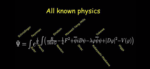
You will see in this theory:
Jake Vanderplass' implementation of the Schrodinger Equation...
"""
General Numerical Solver for the 1D Time-Dependent Schrodinger's equation.

author: Jake Vanderplas
email: vanderplas@astro.washington.edu
website: http://jakevdp.github.com
license: BSD
Please feel free to use and modify this, but keep the above information. Thanks!
"""

import numpy as np
from matplotlib import pyplot as pl
from matplotlib import animation
from scipy.fftpack import fft,ifft


class Schrodinger(object):
    """
    Class which implements a numerical solution of the time-dependent
    Schrodinger equation for an arbitrary potential
    """
    def __init__(self, x, psi_x0, V_x,
                 k0 = None, hbar=1, m=1, t0=0.0):
        """
        Parameters
        ----------
        x : array_like, float
            length-N array of evenly spaced spatial coordinates
        psi_x0 : array_like, complex
            length-N array of the initial wave function at time t0
        V_x : array_like, float
             length-N array giving the potential at each x
        k0 : float
            the minimum value of k.  Note that, because of the workings of the
            fast fourier transform, the momentum wave-number will be defined
            in the range
              k0 < k < 2*pi / dx
            where dx = x[1]-x[0].  If you expect nonzero momentum outside this
            range, you must modify the inputs accordingly.  If not specified,
            k0 will be calculated such that the range is [-k0,k0]
        hbar : float
            value of planck's constant (default = 1)
        m : float
            particle mass (default = 1)
        t0 : float
            initial tile (default = 0)
        """
        # Validation of array inputs
        self.x, psi_x0, self.V_x = map(np.asarray, (x, psi_x0, V_x))
        N = self.x.size
        assert self.x.shape == (N,)
        assert psi_x0.shape == (N,)
        assert self.V_x.shape == (N,)

        # Set internal parameters
        self.hbar = hbar
        self.m = m
        self.t = t0
        self.dt_ = None
        self.N = len(x)
        self.dx = self.x[1] - self.x[0]
        self.dk = 2 * np.pi / (self.N * self.dx)

        # set momentum scale
        if k0 == None:
            self.k0 = -0.5 * self.N * self.dk
        else:
            self.k0 = k0
        self.k = self.k0 + self.dk * np.arange(self.N)

        self.psi_x = psi_x0
        self.compute_k_from_x()

        # variables which hold steps in evolution of the
        self.x_evolve_half = None
        self.x_evolve = None
        self.k_evolve = None

        # attributes used for dynamic plotting
        self.psi_x_line = None
        self.psi_k_line = None
        self.V_x_line = None

    def _set_psi_x(self, psi_x):
        self.psi_mod_x = (psi_x * np.exp(-1j * self.k[0] * self.x)
                          * self.dx / np.sqrt(2 * np.pi))

    def _get_psi_x(self):
        return (self.psi_mod_x * np.exp(1j * self.k[0] * self.x)
                * np.sqrt(2 * np.pi) / self.dx)

    def _set_psi_k(self, psi_k):
        self.psi_mod_k = psi_k * np.exp(1j * self.x[0]
                                        * self.dk * np.arange(self.N))

    def _get_psi_k(self):
        return self.psi_mod_k * np.exp(-1j * self.x[0] *
                                        self.dk * np.arange(self.N))

    def _get_dt(self):
        return self.dt_

    def _set_dt(self, dt):
        if dt != self.dt_:
            self.dt_ = dt
            self.x_evolve_half = np.exp(-0.5 * 1j * self.V_x
                                         / self.hbar * dt )
            self.x_evolve = self.x_evolve_half * self.x_evolve_half
            self.k_evolve = np.exp(-0.5 * 1j * self.hbar /
                                    self.m * (self.k * self.k) * dt)

    psi_x = property(_get_psi_x, _set_psi_x)
    psi_k = property(_get_psi_k, _set_psi_k)
    dt = property(_get_dt, _set_dt)

    def compute_k_from_x(self):
        self.psi_mod_k = fft(self.psi_mod_x)

    def compute_x_from_k(self):
        self.psi_mod_x = ifft(self.psi_mod_k)

    def time_step(self, dt, Nsteps = 1):
        """
        Perform a series of time-steps via the time-dependent
        Schrodinger Equation.

        Parameters
        ----------
        dt : float
            the small time interval over which to integrate
        Nsteps : float, optional
            the number of intervals to compute.  The total change
            in time at the end of this method will be dt * Nsteps.
            default is N = 1
        """
        self.dt = dt

        if Nsteps > 0:
            self.psi_mod_x *= self.x_evolve_half

        for i in range(Nsteps - 1):
            self.compute_k_from_x()
            self.psi_mod_k *= self.k_evolve
            self.compute_x_from_k()
            self.psi_mod_x *= self.x_evolve

        self.compute_k_from_x()
        self.psi_mod_k *= self.k_evolve

        self.compute_x_from_k()
        self.psi_mod_x *= self.x_evolve_half

        self.compute_k_from_x()

        self.t += dt * Nsteps


######################################################################
# Helper functions for gaussian wave-packets

def gauss_x(x, a, x0, k0):
    """
    a gaussian wave packet of width a, centered at x0, with momentum k0
    """
    return ((a * np.sqrt(np.pi)) ** (-0.5)
            * np.exp(-0.5 * ((x - x0) * 1. / a) ** 2 + 1j * x * k0))

def gauss_k(k,a,x0,k0):
    """
    analytical fourier transform of gauss_x(x), above
    """
    return ((a / np.sqrt(np.pi))**0.5
            * np.exp(-0.5 * (a * (k - k0)) ** 2 - 1j * (k - k0) * x0))


######################################################################
# Utility functions for running the animation

def theta(x):
    """
    theta function :
      returns 0 if x<=0, and 1 if x>0
    """
    x = np.asarray(x)
    y = np.zeros(x.shape)
    y[x > 0] = 1.0
    return y

def square_barrier(x, width, height):
    return height * (theta(x) - theta(x - width))

######################################################################
# Create the animation

# specify time steps and duration
dt = 0.01
N_steps = 50
t_max = 120
frames = int(t_max / float(N_steps * dt))

# specify constants
hbar = 1.0   # planck's constant
m = 1.9      # particle mass

# specify range in x coordinate
N = 2 ** 11
dx = 0.1
x = dx * (np.arange(N) - 0.5 * N)

# specify potential
V0 = 1.5
L = hbar / np.sqrt(2 * m * V0)
a = 3 * L
x0 = -60 * L
V_x = square_barrier(x, a, V0)
V_x[x < -98] = 1E6
V_x[x > 98] = 1E6

# specify initial momentum and quantities derived from it
p0 = np.sqrt(2 * m * 0.2 * V0)
dp2 = p0 * p0 * 1./80
d = hbar / np.sqrt(2 * dp2)

k0 = p0 / hbar
v0 = p0 / m
psi_x0 = gauss_x(x, d, x0, k0)

# define the Schrodinger object which performs the calculations
S = Schrodinger(x=x,
                psi_x0=psi_x0,
                V_x=V_x,
                hbar=hbar,
                m=m,
                k0=-28)

######################################################################
# Set up plot
#fig = pl.figure()

# plotting limits
#xlim = (-100, 100)
#klim = (-5, 5)

# top axes show the x-space data
#ymin = 0
#ymax = V0
#ax1 = fig.add_subplot(211, xlim=xlim,
#                      ylim=(ymin - 0.2 * (ymax - ymin),
#                            ymax + 0.2 * (ymax - ymin)))
#psi_x_line, = ax1.plot([], [], c='r', label=r'$|\psi(x)|$')
#V_x_line, = ax1.plot([], [], c='k', label=r'$V(x)$')
#center_line = ax1.axvline(0, c='k', ls=':',
#                          label = r"$x_0 + v_0t$")

#title = ax1.set_title("")
#ax1.legend(prop=dict(size=12))
#ax1.set_xlabel('$x$')
#ax1.set_ylabel(r'$|\psi(x)|$')

# bottom axes show the k-space data
#ymin = abs(S.psi_k).min()
#ymax = abs(S.psi_k).max()
#ax2 = fig.add_subplot(212, xlim=klim,
#                      ylim=(ymin - 0.2 * (ymax - ymin),
#                            ymax + 0.2 * (ymax - ymin)))
#psi_k_line, = ax2.plot([], [], c='r', label=r'$|\psi(k)|$')

#p0_line1 = ax2.axvline(-p0 / hbar, c='k', ls=':', label=r'$\pm p_0$')
#p0_line2 = ax2.axvline(p0 / hbar, c='k', ls=':')
#mV_line = ax2.axvline(np.sqrt(2 * V0) / hbar, c='k', ls='--',
#                      label=r'$\sqrt{2mV_0}$')
#ax2.legend(prop=dict(size=12))
#ax2.set_xlabel('$k$')
#ax2.set_ylabel(r'$|\psi(k)|$')

#V_x_line.set_data(S.x, S.V_x)

######################################################################
# Animate plot
def init():
    psi_x_line.set_data([], [])
    V_x_line.set_data([], [])
    center_line.set_data([], [])

    psi_k_line.set_data([], [])
    title.set_text("")
    return (psi_x_line, V_x_line, center_line, psi_k_line, title)

def animate(i):
    S.time_step(dt, N_steps)
    psi_x_line.set_data(S.x, 4 * abs(S.psi_x))
    V_x_line.set_data(S.x, S.V_x)
    center_line.set_data(2 * [x0 + S.t * p0 / m], [0, 1])

    psi_k_line.set_data(S.k, abs(S.psi_k))
    title.set_text("t = %.2f" % S.t)
    return (psi_x_line, V_x_line, center_line, psi_k_line, title)

# call the animator.  blit=True means only re-draw the parts that have changed.
#anim = animation.FuncAnimation(fig, animate, init_func=init,
#                               frames=frames, interval=30, blit=True)


# uncomment the following line to save the video in mp4 format.  This
# requires either mencoder or ffmpeg to be installed on your system

#anim.save('schrodinger_barrier.mp4', fps=15, extra_args=['-vcodec', 'libx264'])

#display_animation(anim, default_mode='loop')

#anim.save('schrodingerBarrier.gif', writer='imagemagick')
Well, that about does it for things in Physics that we observe, and catches the reader up to the present. Next, let's examine the point particles in our Universe.
Elementary Particles (Work in progress, I hope to implement my own elementary particle explorer in the future)
"Every known elementary particle is identified by its charges with respect to the electromagnetic, weak, strong, and gravitational forces. Electrons have electric charge -1, up quarks 2/3, down quarks -1/3, and neutrinos 0, with antiparticles having opposite electric charges. In the Standard Model these electric charges are a combination of the particles' hypercharge, Y, and weak charge, W.
These charges correspond to the geometry of Lie groups, and unified models of particle physics correspond to how the Lie groups of the Standard Model and gravity embed in larger Lie groups, up to the largest simple exceptional Lie group, E8."
Supersymmetry Breaking
"If supersymmetry is a property of our universe, then it must be broken at an energy that is no lower than 1 TeV, the electroweak symmetry scale. The masses of particles and their superpartners would then no longer be equal, which could explain why no superpartners of known particles have ever been observed."
Time
Imagine you place a pencil on it's tip.
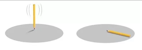
When you let go, the pencil will inevitably fall. When the pencil falls, it provides us with a sense of direction and scale. We can say move an arbitrary number of pencil lengths some arbitrary direction away from the pencil, and end up at a destination relative to the pencil. This is how symmetry breaking works in our Universe.
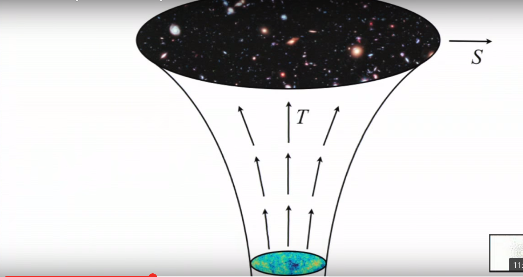
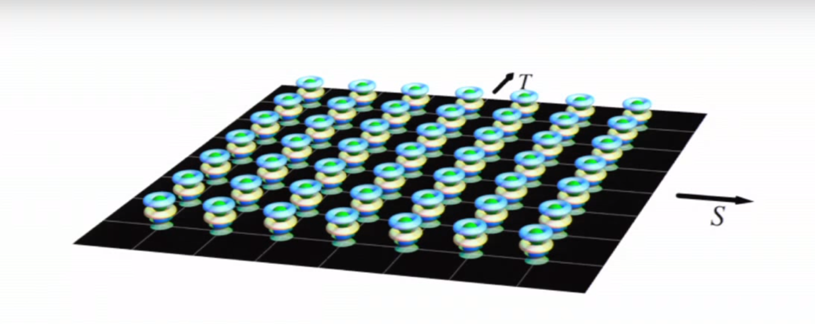
Space is comprised of an X, Y, and Z direction, and exists in the flow of time, T. This gives us the four dimensions we experience as reality. Now imagine this four dimensional fabric of space time without space or time in it.
Let's start by just graphing nothing. In order to graph nothing, we have to decide what nothing means to us. To me, nothing is the absence of matter. In our universe, the framework for this would be our space-time framework, or the 4d fiber we experience as reality. A four dimensional framework roughly means that we need three directions and a unit of time to describe something. At each moment, each of us has a three-dimensional direction and a unit of time in the space-time fiber. Below I wrote a program to display an animation of 3 space and time. This graph has to be an animation for it to make sense to human beings, but we could also create a graph in 3d with color as the fourth dimension.
#Nothing

#An incredible library that converts matplotlib animations to gifs and renderable animations in Ipython
from JSAnimation.IPython_display import display_animation

#Animation libraries and dependencies
import matplotlib.animation as animation
import mpl_toolkits.mplot3d.axes3d as p3


#Define function generator for plane
def generate(X, Y, phi):
    Z = 0
    return Z

#Define our model data
def modelData():
    t_max = 1
    dt = 0.1
    t = 0.0
    x = 0
    y = 0
    z = 0
    while t < t_max:
        t = t + dt
        x = x
        y = y
        z = z
        yield x, y, z, ax, fig, t

#Define our model points
def modelPoints(modelData):
    x, y, z, ax, fig, t = modelData[0], modelData[1], modelData[2], modelData[3], modelData[4], modelData[5]
    return t

#fig = plt.figure()

#ax = p3.Axes3D(fig)

#anim = animation.FuncAnimation(fig, modelPoints, modelData, blit=False, interval=1, repeat=True)

#display_animation(anim, default_mode='once')
#anim.save('Universe.gif', writer='imagemagick')
As you can see, our graph successfully does nothing if we play the animation!
At the "time" of the Big Bang there was a super hot, super dense singularity, and physicists believe that, much like our pencil example, time spontaneously chose a direction and broke symmetry to begin our universe.
Now let's add a 2d grid to our animation to represent a chunk of the space time fiber bundle, and add a length of time.
#SpaceTime
from JSAnimation.IPython_display import display_animation
import matplotlib.animation as animation
import mpl_toolkits.mplot3d.axes3d as p3


#Define function generator for plane
def generate(X, Y, phi):
    Z = 0
    return Z

#Define our model data
def modelData():
    t_max = 10.0
    dt = 0.1
    t = 0.0
    x = 0
    y = 0
    z = 0
    while t < t_max:
        t = t + dt
        x = x
        y = y
        z = z
        yield x, y, z, ax, fig, t

#Define our model points
def modelPoints(modelData):
    x, y, z, ax, fig, t = modelData[0], modelData[1], modelData[2], modelData[3], modelData[4], modelData[5]
    ax.cla()
    Z = generate(X, Y, 0)
    wframe = ax.plot_wireframe(X, Y, Z, rstride=2, cstride=2, color = "black")
    ax.set_xlim(-1, 1)
    ax.set_ylim(-1, 1)
    ax.set_zlim(-1, 1)
    return wframe

#fig = plt.figure()

#ax = p3.Axes3D(fig)

#xs = np.linspace(-1, 1, 50)

#ys = np.linspace(-1, 1, 50)

#X, Y = np.meshgrid(xs, ys)

#Z = generate(X, Y, 0.0)

#anim = animation.FuncAnimation(fig, modelPoints, modelData, blit=False, interval=20, repeat=True)

#display_animation(anim, default_mode='once')
#anim.save('SpaceTime.gif', writer='imagemagick')
When this singularity chose a direction for the flow of time, it spewed its contents in that direction, and if we fast-forward approximately fourteen billion years, we have the conditions for matter, and if we move perpendicular in space to the flow of time, we arrive at a tiny blue planet called Earth.

--Image courtesy of NASA
As Garrett Lisi explains in his Ted Talk on particle physics however,
"The flow of time is not linear. Matter actually bends time and causes time to ripple, we observe these ripples as gravitational waves. In fact, the Earth is so dense that it actually bends the flow of time towards it's center to give us the gravity that keeps us from flying into space!"
So what is this matter stuff...
According to Lisi,
"At each point in space time there is another internal space, with many dimensions, that are perpendicular to our three dimensions of space X, Y, and Z. This internal space is attached to space time and moves over it. For each different direction in this inner space, there is a corresponding different kind of elementary particle that can exist at a point in space time!"
Electroweak symmetry breaking and the quark epoch
"As the universe's temperature falls below a certain very high energy level, it is believed that the Higgs field spontaneously acquires a vacuum expectation value, which breaks electroweak gauge symmetry. This has two related effects:
The weak force and electromagnetic force, and their respective bosons (the W and Z bosons and photon) manifest differently in the present universe, with different ranges; Via the Higgs mechanism, all elementary particles interacting with the Higgs field become massive, having been massless at higher energy levels. At the end of this epoch, the fundamental interactions of gravitation, electromagnetism, the strong interaction and the weak interaction have now taken their present forms, and fundamental particles have mass, but the temperature of the universe is still too high to allow quarks to bind together to form hadrons."
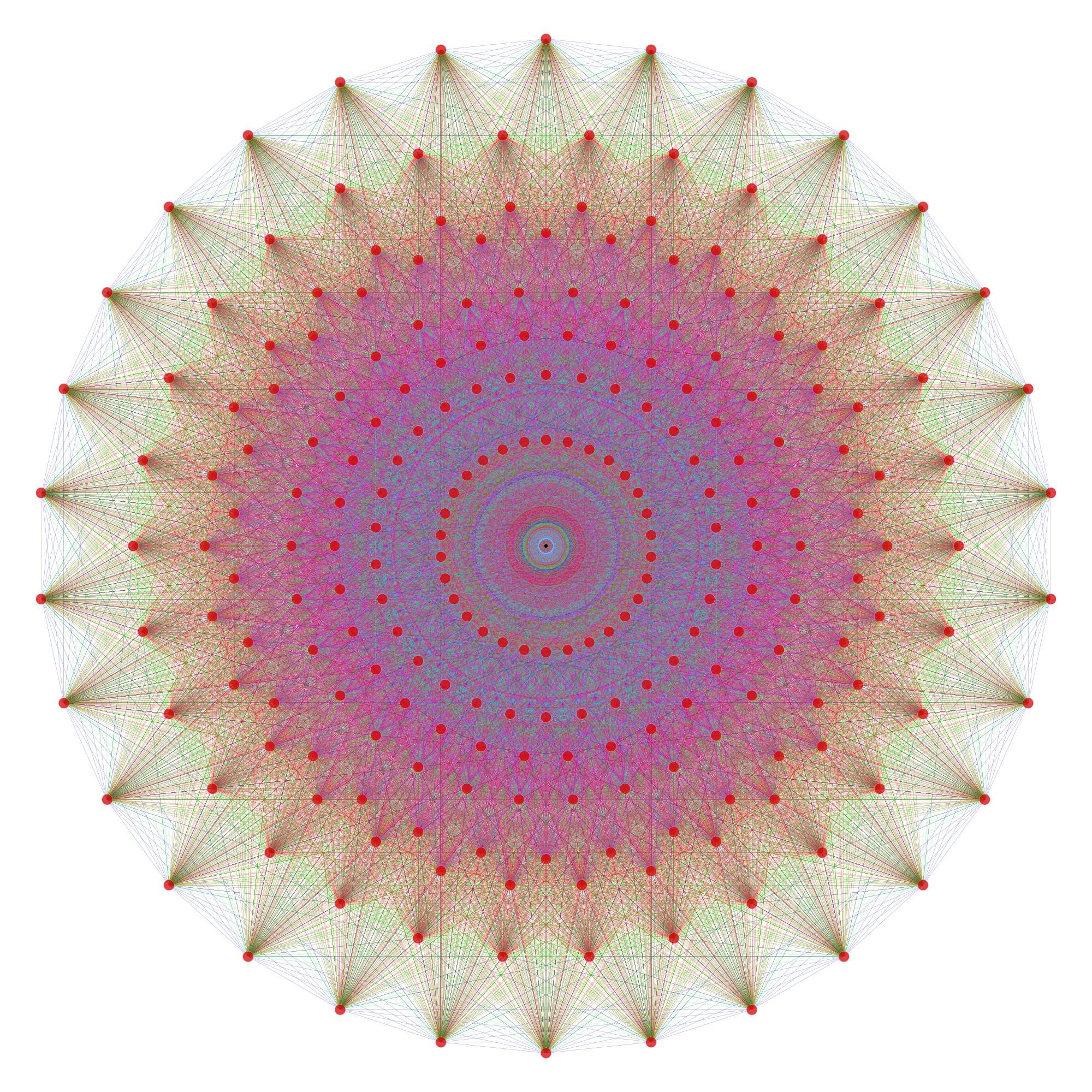
Higgs Field
Lisi goes on in his Ted Talk to explain how the higgs field give the massive particles their mass, and does a great job describing how all elementary particles exist together in one sacred geometrical figure, the E8 Lie Group.
#Symmetry Breaking
from JSAnimation.IPython_display import display_animation
import matplotlib.animation as animation
import mpl_toolkits.mplot3d.axes3d as p3


#Define function generator for plane
def generate(X, Y, theta):
    Z = .5*(np.cos(np.pi*np.sqrt((X**2)+(Y**2))))
    return Z

#Define our model data
def modelData():
    t_max = 10.0
    dt = 0.1
    t = 0.0
    x = 0
    y = 0
    z = .5
    while t < t_max:
        t = t + dt
        x = x
        y = y
        z = z
        yield x, y, z, ax, fig, t

#Define our model points
def modelPoints(modelData):
    x, y, z, ax, fig, t = modelData[0], modelData[1], modelData[2], modelData[3], modelData[4], modelData[5]
    ax.cla()
    theta = t
    xs = np.linspace(-1, 1, 50)
    ys = np.linspace(-1, 1, 50)
    X, Y = np.meshgrid(xs, ys)
    Z = generate(X, Y, theta)
    wframe = ax.plot_wireframe(X, Y, Z, rstride=2, cstride=2, color = "black")
    line1, = ax.plot([x], [y], [z],'bo', ms=20)
    x = x + np.exp(t)/22026
    y = y + np.exp(t)/22026
    z = .5*(np.cos(np.pi*np.sqrt((x**2)+(y**2))))
    line1.set_data(x, y)
    line1.set_3d_properties(z)
    ax.set_xlim(-1, 1)
    ax.set_ylim(-1, 1)
    ax.set_zlim(-1, 1)
    return wframe, line1

#fig = plt.figure()

#ax = p3.Axes3D(fig)

#anim = animation.FuncAnimation(fig, modelPoints, modelData, blit=False, interval=20, repeat=True)

#display_animation(anim, default_mode='once')
#anim.save('SymmetryBreaking.gif', writer='imagemagick')
"One very important part of this inner space are the four dimensions corresponding to the Higgs Field. Imagine the balls above to be perfectly smooth, 4d surfaces. Via symmetry breaking, we choose one direction to be special. This is very similar to how the flow of time becomes special in space time, but we are dealing with the internal space of particle physics now."
#Higgs
from JSAnimation.IPython_display import display_animation
import matplotlib.animation as animation
import mpl_toolkits.mplot3d.axes3d as p3


#Define function generator for plane
def generate(X, Y, phi):
    Z = 0
    return Z

#Define our model data
def modelData():
    t_max = 10
    dt = 0.1
    t = 0.0
    x = 0
    y = 0
    z = 0
    while t < t_max:
        t = t + dt
        x = x
        y = y
        z = z
        yield x, y, z, ax, fig, t

#Define our model points
def modelPoints(modelData):
    x, y, z, ax, fig, t = modelData[0], modelData[1], modelData[2], modelData[3], modelData[4], modelData[5]
    if t >= 9.8:
        line1, = ax.plot([x], [y], [z],'bo', ms=100)
        line1.set_data(x, y)
        line1.set_3d_properties(z)
        line2, = ax.plot([x], [y], [z],'w^', ms=50)
        line2.set_data(x, y)
        line2.set_3d_properties(z+.25)
        ax.set_xlim(-1, 1)
        ax.set_ylim(-1, 1)
        ax.set_zlim(-1, 1)
        return t, line1, line2
    else:
        line1, = ax.plot([x], [y], [z],'bo', ms=100)
        line1.set_data(x, y)
        line1.set_3d_properties(z)
        ax.set_xlim(-1, 1)
        ax.set_ylim(-1, 1)
        ax.set_zlim(-1, 1)
        return t, line1

#fig = plt.figure()

#ax = p3.Axes3D(fig)

#anim = animation.FuncAnimation(fig, modelPoints, modelData, blit=False, interval=10, repeat=True)

#display_animation(anim, default_mode='once')
#anim.save('Higgs.gif', writer='imagemagick')
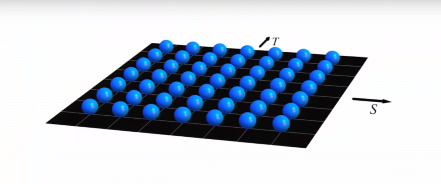
"With the higgs direction picked out, we now have what is referred to as the Higgs Background."
#Higgs Field
from JSAnimation.IPython_display import display_animation
import matplotlib.animation as animation
import mpl_toolkits.mplot3d.axes3d as p3


#Define function generator for plane
def generate(X, Y, phi):
    Z = 0
    return Z

#Define our model data
def modelData():
    t_max = 10.0
    dt = 0.1
    t = 0.0
    x = 0
    y = 0
    z = 0
    while t < t_max:
        t = t + dt
        x = x
        y = y
        z = z
        yield x, y, z, ax, fig, t

#Define our model points
def modelPoints(modelData):
    x, y, z, ax, fig, t = modelData[0], modelData[1], modelData[2], modelData[3], modelData[4], modelData[5]
    if t >= 9.8:
        ax.cla()
        Z = generate(X, Y, 0)
        wframe = ax.plot_wireframe(X, Y, Z, rstride=2, cstride=2, color = "black")
        line1, = ax.plot([x], [y], [z],'bo', ms=10)
        line1.set_data(x-1, y-1)
        line1.set_3d_properties(z)
        line2, = ax.plot([x], [y], [z],'bo', ms=10)
        line2.set_data(x-.5, y-1)
        line2.set_3d_properties(z)
        line3, = ax.plot([x], [y], [z],'bo', ms=10)
        line3.set_data(x, y-1)
        line3.set_3d_properties(z)
        line4, = ax.plot([x], [y], [z],'bo', ms=10)
        line4.set_data(x+.5, y-1)
        line4.set_3d_properties(z)
        line5, = ax.plot([x], [y], [z],'bo', ms=10)
        line5.set_data(x+1, y-1)
        line5.set_3d_properties(z)
        line6, = ax.plot([x], [y], [z],'bo', ms=10)
        line6.set_data(x-1, y-.5)
        line6.set_3d_properties(z)
        line7, = ax.plot([x], [y], [z],'bo', ms=10)
        line7.set_data(x-.5, y-.5)
        line7.set_3d_properties(z)
        line8, = ax.plot([x], [y], [z],'bo', ms=10)
        line8.set_data(x, y-.5)
        line8.set_3d_properties(z)
        line9, = ax.plot([x], [y], [z],'bo', ms=10)
        line9.set_data(x+.5, y-.5)
        line9.set_3d_properties(z)
        line10, = ax.plot([x], [y], [z],'bo', ms=10)
        line10.set_data(x+1, y-.5)
        line10.set_3d_properties(z)
        line11, = ax.plot([x], [y], [z],'bo', ms=10)
        line11.set_data(x-1, y)
        line11.set_3d_properties(z)
        line12, = ax.plot([x], [y], [z],'bo', ms=10)
        line12.set_data(x-.5, y)
        line12.set_3d_properties(z)
        line13, = ax.plot([x], [y], [z],'bo', ms=10)
        line13.set_data(x, y)
        line13.set_3d_properties(z)
        line14, = ax.plot([x], [y], [z],'bo', ms=10)
        line14.set_data(x+.5, y)
        line14.set_3d_properties(z)
        line15, = ax.plot([x], [y], [z],'bo', ms=10)
        line15.set_data(x+1, y)
        line15.set_3d_properties(z)
        line16, = ax.plot([x], [y], [z],'bo', ms=10)
        line16.set_data(x-1, y+.5)
        line16.set_3d_properties(z)
        line17, = ax.plot([x], [y], [z],'bo', ms=10)
        line17.set_data(x-.5, y+.5)
        line17.set_3d_properties(z)
        line18, = ax.plot([x], [y], [z],'bo', ms=10)
        line18.set_data(x, y+.5)
        line18.set_3d_properties(z)
        line19, = ax.plot([x], [y], [z],'bo', ms=10)
        line19.set_data(x+.5, y+.5)
        line19.set_3d_properties(z)
        line20, = ax.plot([x], [y], [z],'bo', ms=10)
        line20.set_data(x+1, y+.5)
        line20.set_3d_properties(z)
        line21, = ax.plot([x], [y], [z],'bo', ms=10)
        line21.set_data(x-1, y+1)
        line21.set_3d_properties(z)
        line22, = ax.plot([x], [y], [z],'bo', ms=10)
        line22.set_data(x-.5, y+1)
        line22.set_3d_properties(z)
        line23, = ax.plot([x], [y], [z],'bo', ms=10)
        line23.set_data(x, y+1)
        line23.set_3d_properties(z)
        line24, = ax.plot([x], [y], [z],'bo', ms=10)
        line24.set_data(x+.5, y+1)
        line24.set_3d_properties(z)
        line25, = ax.plot([x], [y], [z],'bo', ms=10)
        line25.set_data(x+1, y+1)
        line25.set_3d_properties(z)
        line26, = ax.plot([x], [y], [z],'w^', ms=5)
        line26.set_data(x-1, y-1)
        line26.set_3d_properties(z)
        line27, = ax.plot([x], [y], [z],'w^', ms=5)
        line27.set_data(x-.5, y-1)
        line27.set_3d_properties(z)
        line28, = ax.plot([x], [y], [z],'w^', ms=5)
        line28.set_data(x, y-1)
        line28.set_3d_properties(z)
        line29, = ax.plot([x], [y], [z],'w^', ms=5)
        line29.set_data(x+.5, y-1)
        line29.set_3d_properties(z)
        line30, = ax.plot([x], [y], [z],'w^', ms=5)
        line30.set_data(x+1, y-1)
        line30.set_3d_properties(z)
        line31, = ax.plot([x], [y], [z],'w^', ms=5)
        line31.set_data(x-1, y-.5)
        line31.set_3d_properties(z)
        line32, = ax.plot([x], [y], [z],'w^', ms=5)
        line32.set_data(x-.5, y-.5)
        line32.set_3d_properties(z)
        line33, = ax.plot([x], [y], [z],'w^', ms=5)
        line33.set_data(x, y-.5)
        line33.set_3d_properties(z)
        line34, = ax.plot([x], [y], [z],'w^', ms=5)
        line34.set_data(x+.5, y-.5)
        line34.set_3d_properties(z)
        line35, = ax.plot([x], [y], [z],'w^', ms=5)
        line35.set_data(x+1, y-.5)
        line35.set_3d_properties(z)
        line36, = ax.plot([x], [y], [z],'w^', ms=5)
        line36.set_data(x-1, y)
        line36.set_3d_properties(z)
        line37, = ax.plot([x], [y], [z],'w^', ms=5)
        line37.set_data(x-.5, y)
        line37.set_3d_properties(z)
        line38, = ax.plot([x], [y], [z],'w^', ms=5)
        line38.set_data(x, y)
        line38.set_3d_properties(z)
        line39, = ax.plot([x], [y], [z],'w^', ms=5)
        line39.set_data(x+.5, y)
        line39.set_3d_properties(z)
        line40, = ax.plot([x], [y], [z],'w^', ms=5)
        line40.set_data(x+1, y)
        line40.set_3d_properties(z)
        line41, = ax.plot([x], [y], [z],'w^', ms=5)
        line41.set_data(x-1, y+.5)
        line41.set_3d_properties(z)
        line42, = ax.plot([x], [y], [z],'w^', ms=5)
        line42.set_data(x-.5, y+.5)
        line42.set_3d_properties(z)
        line43, = ax.plot([x], [y], [z],'w^', ms=5)
        line43.set_data(x, y+.5)
        line43.set_3d_properties(z)
        line44, = ax.plot([x], [y], [z],'w^', ms=5)
        line44.set_data(x+.5, y+.5)
        line44.set_3d_properties(z)
        line45, = ax.plot([x], [y], [z],'w^', ms=5)
        line45.set_data(x+1, y+.5)
        line45.set_3d_properties(z)
        line46, = ax.plot([x], [y], [z],'w^', ms=5)
        line46.set_data(x-1, y+1)
        line46.set_3d_properties(z)
        line47, = ax.plot([x], [y], [z],'w^', ms=5)
        line47.set_data(x-.5, y+1)
        line47.set_3d_properties(z)
        line48, = ax.plot([x], [y], [z],'w^', ms=5)
        line48.set_data(x, y+1)
        line48.set_3d_properties(z)
        line49, = ax.plot([x], [y], [z],'w^', ms=5)
        line49.set_data(x+.5, y+1)
        line49.set_3d_properties(z)
        line50, = ax.plot([x], [y], [z],'w^', ms=5)
        line50.set_data(x+1, y+1)
        line50.set_3d_properties(z)
        ax.set_xlim(-1, 1)
        ax.set_ylim(-1, 1)
        ax.set_zlim(-1, 1)
        return line1, line2, line3, line4, line5,
        line6, line7, line8, line9, line10, line11, line12,
        line13, line14, line15, line16, line17, line18,
        line19, line20, line21, line22, line23, line24,
        line25, line26, line27, line28, line29, line30,
        line31, line32, line33, line34, line35, line36,
        line37, line38, line39, line40, line41, line42,
        line43, line44, line45, line46, line47, line48,
        line49, line50, wframe
    else:
        ax.cla()
        Z = generate(X, Y, 0)
        line1, = ax.plot([x], [y], [z],'bo', ms=10)
        line1.set_data(x-1, y-1)
        line1.set_3d_properties(z)
        line2, = ax.plot([x], [y], [z],'bo', ms=10)
        line2.set_data(x-.5, y-1)
        line2.set_3d_properties(z)
        line3, = ax.plot([x], [y], [z],'bo', ms=10)
        line3.set_data(x, y-1)
        line3.set_3d_properties(z)
        line4, = ax.plot([x], [y], [z],'bo', ms=10)
        line4.set_data(x+.5, y-1)
        line4.set_3d_properties(z)
        line5, = ax.plot([x], [y], [z],'bo', ms=10)
        line5.set_data(x+1, y-1)
        line5.set_3d_properties(z)
        line6, = ax.plot([x], [y], [z],'bo', ms=10)
        line6.set_data(x-1, y-.5)
        line6.set_3d_properties(z)
        line7, = ax.plot([x], [y], [z],'bo', ms=10)
        line7.set_data(x-.5, y-.5)
        line7.set_3d_properties(z)
        line8, = ax.plot([x], [y], [z],'bo', ms=10)
        line8.set_data(x, y-.5)
        line8.set_3d_properties(z)
        line9, = ax.plot([x], [y], [z],'bo', ms=10)
        line9.set_data(x+.5, y-.5)
        line9.set_3d_properties(z)
        line10, = ax.plot([x], [y], [z],'bo', ms=10)
        line10.set_data(x+1, y-.5)
        line10.set_3d_properties(z)
        line11, = ax.plot([x], [y], [z],'bo', ms=10)
        line11.set_data(x-1, y)
        line11.set_3d_properties(z)
        line12, = ax.plot([x], [y], [z],'bo', ms=10)
        line12.set_data(x-.5, y)
        line12.set_3d_properties(z)
        line13, = ax.plot([x], [y], [z],'bo', ms=10)
        line13.set_data(x, y)
        line13.set_3d_properties(z)
        line14, = ax.plot([x], [y], [z],'bo', ms=10)
        line14.set_data(x+.5, y)
        line14.set_3d_properties(z)
        line15, = ax.plot([x], [y], [z],'bo', ms=10)
        line15.set_data(x+1, y)
        line15.set_3d_properties(z)
        line16, = ax.plot([x], [y], [z],'bo', ms=10)
        line16.set_data(x-1, y+.5)
        line16.set_3d_properties(z)
        line17, = ax.plot([x], [y], [z],'bo', ms=10)
        line17.set_data(x-.5, y+.5)
        line17.set_3d_properties(z)
        line18, = ax.plot([x], [y], [z],'bo', ms=10)
        line18.set_data(x, y+.5)
        line18.set_3d_properties(z)
        line19, = ax.plot([x], [y], [z],'bo', ms=10)
        line19.set_data(x+.5, y+.5)
        line19.set_3d_properties(z)
        line20, = ax.plot([x], [y], [z],'bo', ms=10)
        line20.set_data(x+1, y+.5)
        line20.set_3d_properties(z)
        line21, = ax.plot([x], [y], [z],'bo', ms=10)
        line21.set_data(x-1, y+1)
        line21.set_3d_properties(z)
        line22, = ax.plot([x], [y], [z],'bo', ms=10)
        line22.set_data(x-.5, y+1)
        line22.set_3d_properties(z)
        line23, = ax.plot([x], [y], [z],'bo', ms=10)
        line23.set_data(x, y+1)
        line23.set_3d_properties(z)
        line24, = ax.plot([x], [y], [z],'bo', ms=10)
        line24.set_data(x+.5, y+1)
        line24.set_3d_properties(z)
        line25, = ax.plot([x], [y], [z],'bo', ms=10)
        line25.set_data(x+1, y+1)
        line25.set_3d_properties(z)
        wframe = ax.plot_wireframe(X, Y, Z, rstride=2, cstride=2, color = "black")
        ax.set_xlim(-1, 1)
        ax.set_ylim(-1, 1)
        ax.set_zlim(-1, 1)
        return line1, line2, line3, line4, line5, line6,
        line7, line8, line9, line10, line11, line12,
        line13, line14, line15, line16, line17, line18,
        line19, line20, line21, line22, line23, line24,
        line25, wframe

#fig = plt.figure()

#ax = p3.Axes3D(fig)

#xs = np.linspace(-1, 1, 50)

#ys = np.linspace(-1, 1, 50)

#X, Y = np.meshgrid(xs, ys)

#Z = generate(X, Y, 0.0)

#anim = animation.FuncAnimation(fig, modelPoints, modelData, blit=True, interval=20, repeat=True)

#display_animation(anim, default_mode='once')

#anim.save('HiggsField.gif', writer='imagemagick')
"Just like time can ripple, this Higgs Field can also ripple. A ripple, in the direction of the Higgs Field over space time, creates what we see as a Higgs Boson! This particle has actually been popped into existence in the Large Hadron Collider at Geneva."
"To understand how this validated theory explains how particles get mass, you have to understand how the Higgs shape twists around the inner space of elementary particles, specifically in regards to the Electroweak Force..."
"Enter the Strong Nuclear Force, the Electroweak Force, and Gravity!"
-Ted X Maui,Garrett Lixi
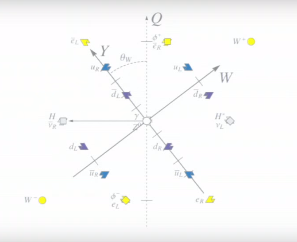
Electroweak Force
"The Electroweak Force is comprised of weak charge, W and hypercharge, γ."
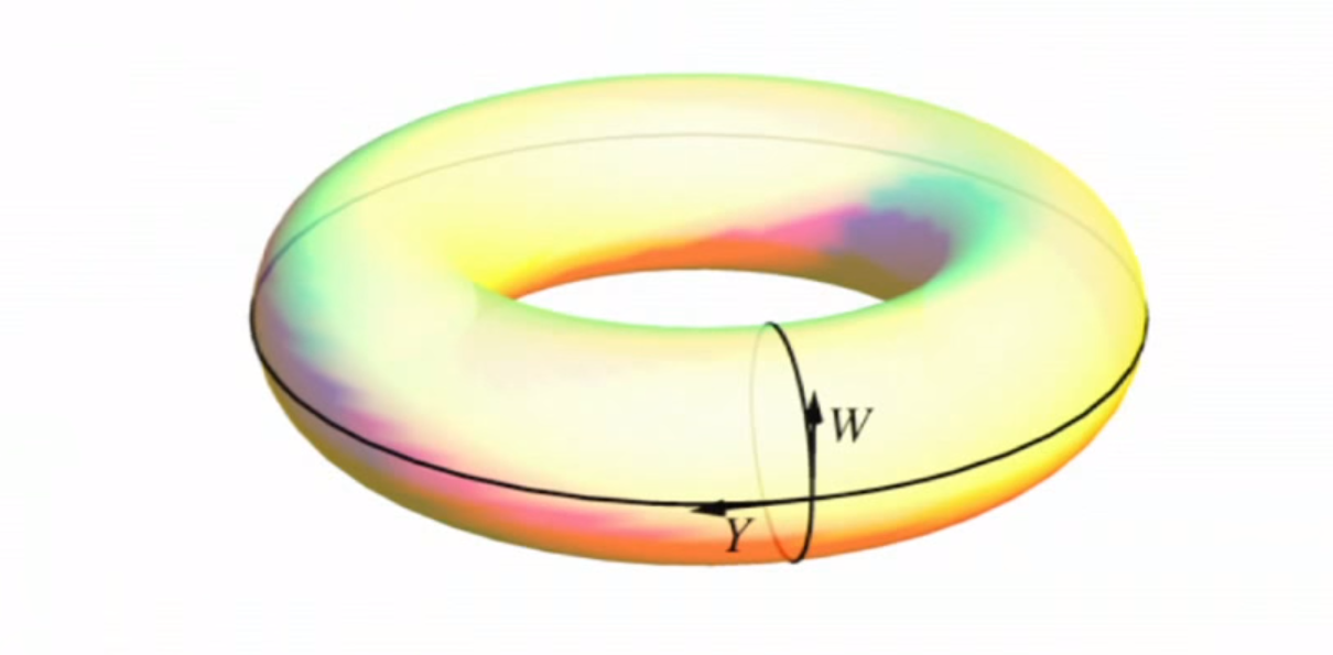
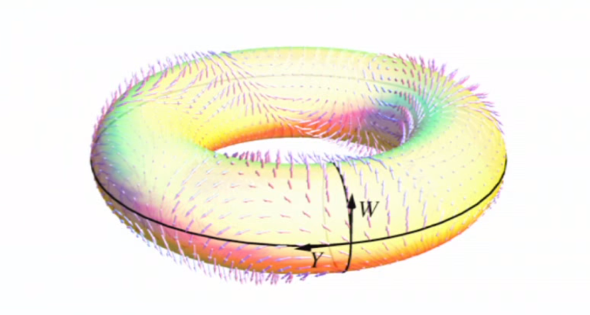
"The Higgs direction is not uniform along this electroweak torus, it actually twists around it. These twists correspond to the charges of that Higgs direction."
#ElectroWeakTorusHiggs
from JSAnimation.IPython_display import display_animation
import matplotlib.animation as animation
import mpl_toolkits.mplot3d.axes3d as p3


#Define function generator for plane
def generate(X, Y, Z):

    return Z

#Define our model data
def modelData():
    t_max = 20.0
    dt = .2
    t = 0.0
    x = 0
    y = 0
    z = 0
    while t < t_max:
        t = t + dt
        x = x
        y = y
        z = z
        yield x, y, z, ax, fig, t

#Define our model points
def modelPoints(modelData):
    x, y, z, ax, fig, t = modelData[0], modelData[1], modelData[2], modelData[3], modelData[4], modelData[5]
    ax.cla()
    Z = generate(X, Y, 0)
    c, a = 2, 1
    x = ((c + a*np.cos(theta)) * np.cos(phi))/np.pi
    y = ((c + a*np.cos(theta)) * np.sin(phi))/np.pi
    z = (a * np.sin(theta))/np.pi
    wframe = ax.plot_wireframe(x, y, z, rstride=2, cstride=2, color = "yellow")
    x = (((c + a*np.cos(2*np.pi+t/2)) * np.cos(2*np.pi+t/2))/np.pi)
    y = (((c + a*np.cos(2*np.pi+t/2)) * np.sin(2*np.pi+t/2))/np.pi)
    z = ((a * np.sin(2 * np.pi+t/2))/np.pi)
    line, = ax.plot([x], [y], [z],'bo', ms=20)
    ax.set_xlim(-1, 1)
    ax.set_ylim(-1, 1)
    ax.set_zlim(-1, 1)
    return wframe, line

#fig = plt.figure()

#ax = p3.Axes3D(fig)

#n = 100

#theta = np.linspace(0, 2.*np.pi, n)
#phi = np.linspace(0, 2.*np.pi, n)
#theta, phi = np.meshgrid(theta, phi)

#anim = animation.FuncAnimation(fig, modelPoints, modelData, blit=False, interval=20, repeat=True)

#display_animation(anim, default_mode='reflect')
#anim.save('ElectroWeakTorusHiggs.gif', writer='imagemagick')
"Although this geometry is very complicated, you can simply count the number of twists the Higgs Field makes around the torus, and plot them relative to the weak charge and hypercharge to form a nice graph."
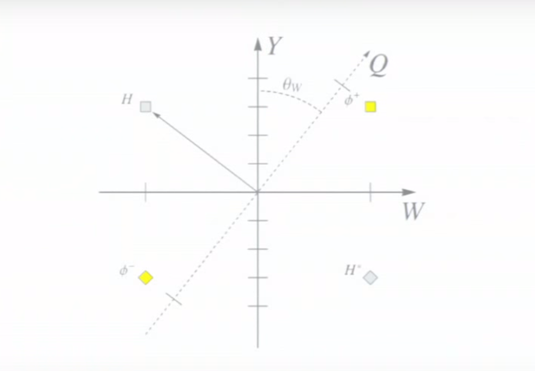
"This is how the symmetry of the Electroweak force gets broken. Perpendicular to this Higgs direction is what we call Electric Charge, which makes an angle called the weak mixing angle, and this Electric Charge is made of part hypercharge, and part weak charge. All of the other elementary particles that we know of can be plotted relative to their twists around the Electroweak torus, and we can plot them according to these twists and see their charges."
![]()
"Here is our graph of the weak charge and hypercharge."
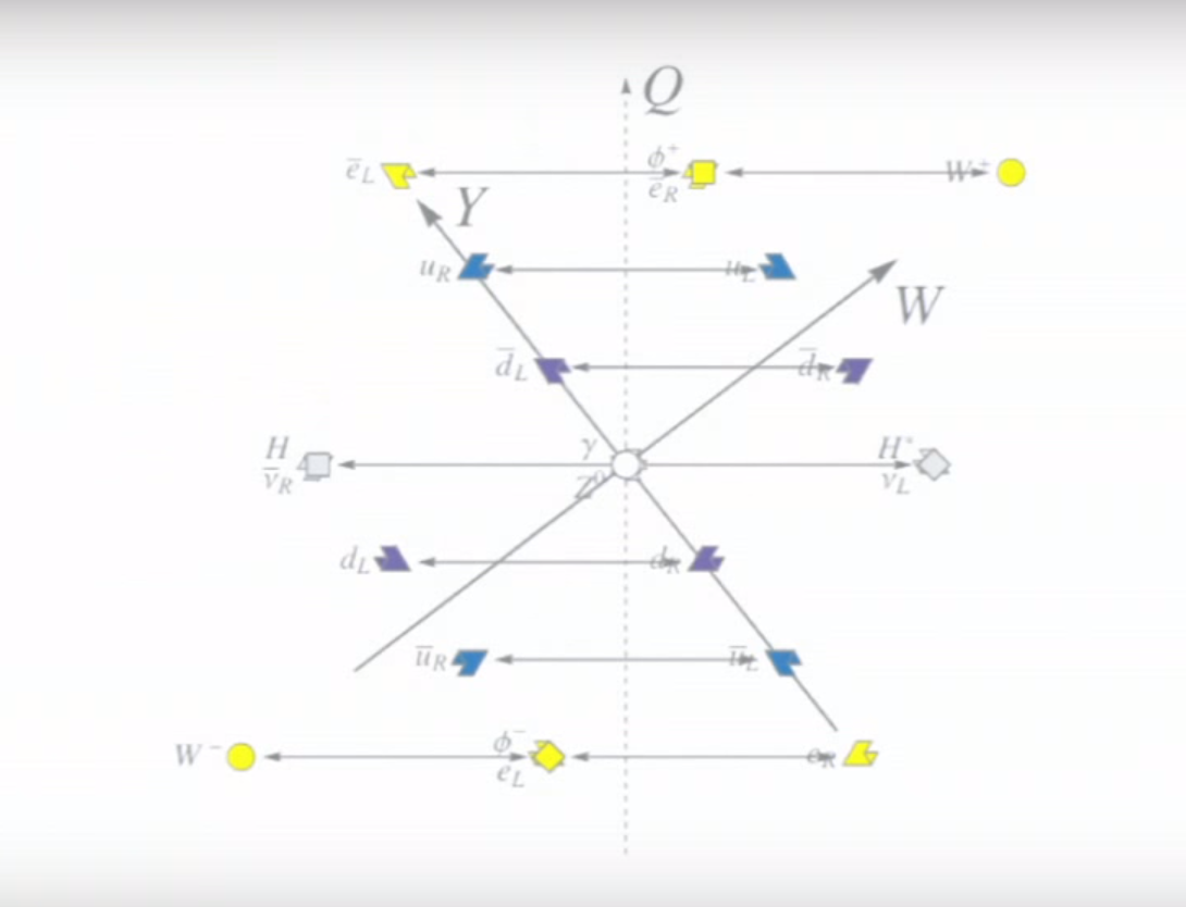
"Here is the graph with the three components of the Higgs Field added in."
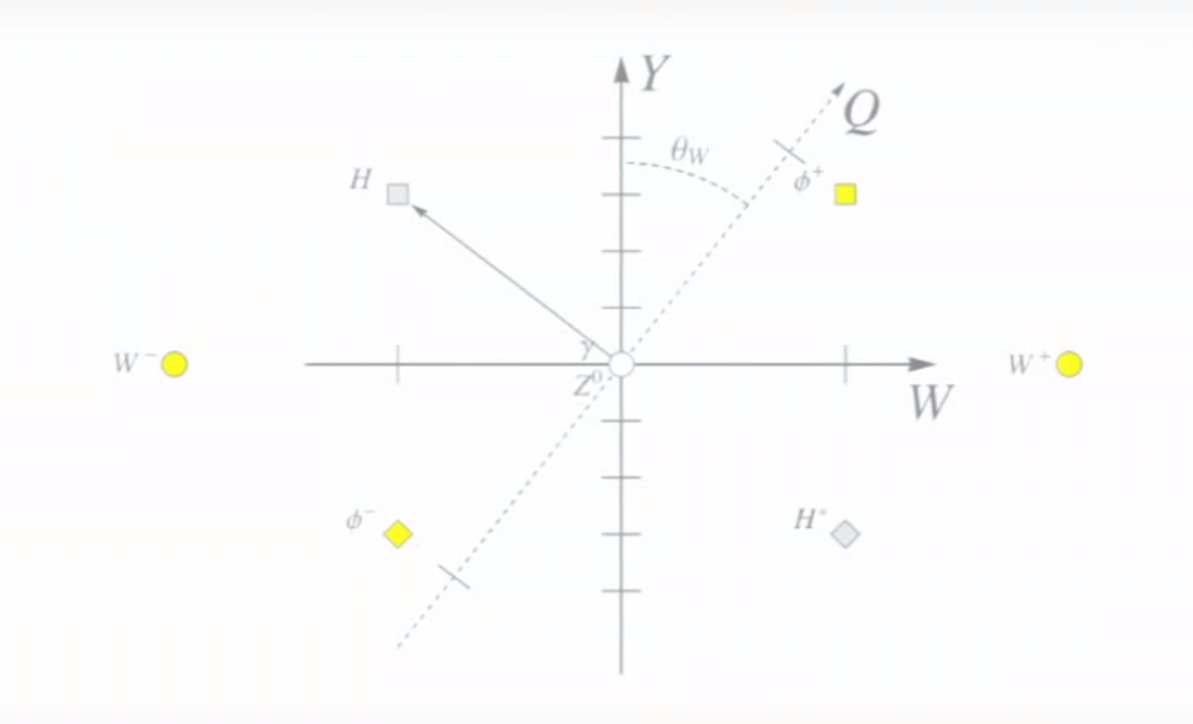
"The W Bosons.(The photons and Z0 do not twist, they are parallel around this torus; so they sit in the center of this diagram)."
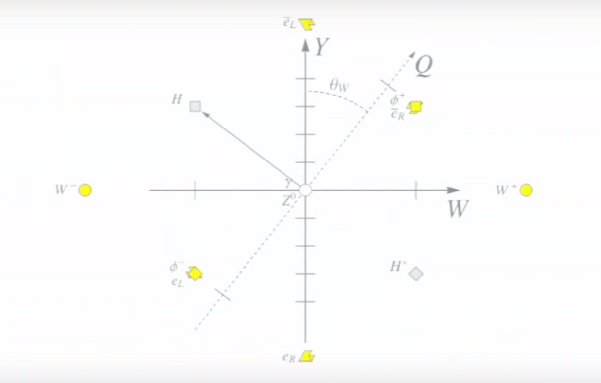
"The electron, which has four different parts, its left and right part, and the particle and antiparticle."
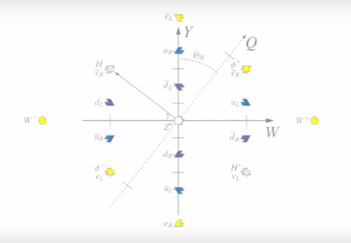
"The quarks and neutrinos also have four parts."
"By now you should have picked up on the fundamental pattern of our universe. There are other particles you may have heard of, such as the bottom and top quarks, but they have the same number of twists as the up and down quarks so there is alot of overlap."
"You can rotate this diagram by the weak mixing angle, and see how the Higgs particle interacts with all of these particles to give them their mass!"
"Let's examine the graph with the Higgs direction added in. As an example, the Higgs direction, when added to the right handed part of the electron, turns into the left handed part of the electron. What is happening is, at each point in space time there is an electron, the electron is bouncing back and forth between it's left and righthanded parts interacting with the Higgs Background to give it mass!"
"This happens for every other massive particle, giving us all of the elementary particles we see!"
-Ted X Maui,Garrett Lixi
Strong Nuclear Force
"As we mentioned earlier, inside this internal elementary particle space, there is another force called the Strong Nuclear force. The strong force is what hold the atoms nucleus together and The strong Nuclear force can also be modeled as a torus, and gravity can be viewed as a hyperbolic torus."
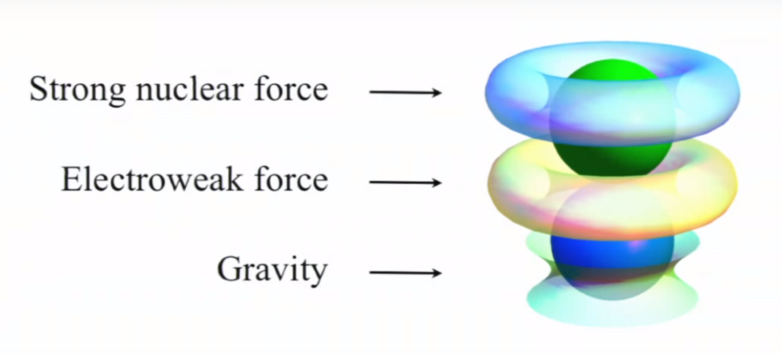
"The quarks also twist around the Strong Nuclear Force torus as well, which creates color charge. Gluons also twist around the strong Torus and carry the strong force. When they interact with the quarks, they change their color, and this is what binds quarks together to give us the atomic nuclei."
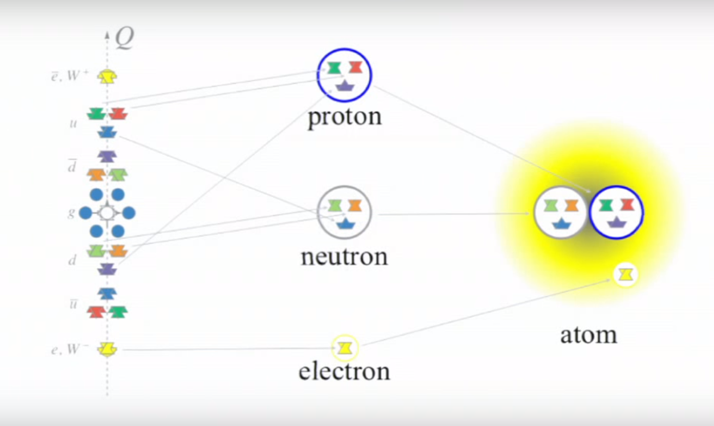
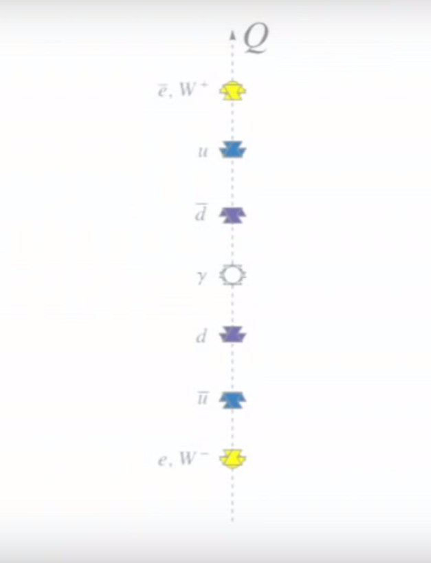
"This is how all the matter we know of in the Universe comes to exist...
A down quark and two up quarks make a proton of total electric charge +1,
An up quark and two down quarks make a neutron with total electric charge of zero,
These clump together, bound by the strong force, orbited by electrons, bound by photons, and we see Everything around us in the Universe. All of this described by a sacred geometry."
-Ted X Maui,Garrett Lixi
Life
Habitable epoch
"The chemistry of life may have begun shortly after the Big Bang, 13.8 billion years ago, during a habitable epoch when the Universe was only 10-17 million years old."
Structural Formation
"Structure formation in the big bang model proceeds hierarchically, with smaller structures forming before larger ones. The first structures to form are quasars, which are thought to be bright, early active galaxies, and population III stars. Before this epoch, the evolution of the universe could be understood through linear cosmological perturbation theory: that is, all structures could be understood as small deviations from a perfect homogeneous universe. This is computationally relatively easy to study. At this point non-linear structures begin to form, and the computational problem becomes much more difficult, involving, for example, N-body simulations with billions of particles."
Reionization
"The first stars and quasars form from gravitational collapse. The intense radiation they emit reionizes the surrounding universe. From this point on, most of the universe is composed of plasma."
Formation of Stars
"The first stars, most likely Population III stars, form and start the process of turning the light elements that were formed in the Big Bang (hydrogen, helium and lithium) into heavier elements. However, as yet there have been no observed Population III stars, and understanding of them is currently based on computational models of their formation and evolution. Fortunately observations of the Cosmic Microwave Background radiation can be used to date when star formation began in earnest. Analysis of such observations made by the European Space Agency's Planck telescope, as reported by BBC News in early February, 2015, concludes that the first generation of stars lit up 560 million years after the Big Bang."
Formation of Galaxies
"Large volumes of matter collapse to form a galaxy. Population II stars are formed early on in this process, with Population I stars formed later.
Johannes Schedler's project has identified a quasar CFHQS 1641+3755 at 12.7 billion light-years away, when the universe was just 7% of its present age.
On July 11, 2007, using the 10-metre Keck II telescope on Mauna Kea, Richard Ellis of the California Institute of Technology at Pasadena and his team found six star forming galaxies about 13.2 billion light years away and therefore created when the universe was only 500 million years old. Only about 10 of these extremely early objects are currently known. More recent observations have shown these ages to be shorter than previously indicated. The most distant galaxy observed as of October 2013 has been reported to be 13.1 billion light years away.
The Hubble Ultra Deep Field shows a number of small galaxies merging to form larger ones, at 13 billion light years, when the universe was only 5% its current age. This age estimate is now believed to be slightly shorter.
Based upon the emerging science of nucleocosmochronology, the Galactic thin disk of the Milky Way is estimated to have been formed 8.8 ± 1.7 billion years ago."
Formation of Groups, Clusters and Superclusters
"Gravitational attraction pulls galaxies towards each other to form groups, clusters and superclusters."
Formation of the Solar System
"The Solar System began forming about 4.6 billion years ago, or about 9 billion years after the Big Bang. A fragment of a molecular cloud made mostly of hydrogen and traces of other elements began to collapse, forming a large sphere in the center which would become the Sun, as well as a surrounding disk. The surrounding accretion disk would coalesce into a multitude of smaller objects that would become planets, asteroids, and comets. The Sun is a late-generation star, and the Solar System incorporates matter created by previous generations of stars."